Just recently some friends at work have started playing Magic The Gathering again.  MTG was one of the first collectible card games from Wizards of the Coast. I got a bit hooked on it back in the late 90’s and used to play quite a lot with friends.  The “official” definition from Wikipedia goes as follows:

Each game represents a battle between powerful wizards, known as “planeswalkers“, who use the magical spells, items, and fantastic creatures depicted on individual Magic cards to defeat their opponents. Although the original concept of the game drew heavily from the motifs of traditional fantasy role-playing games such as Dungeons & Dragons, the gameplay of Magic bears little resemblance to pencil-and-paper adventure games, while having substantially more cards and more complex rules than many other card games.

There’s even a YouTube channel that teaches you how to play!

Honestly, it’s not nearly as geeky as it sounds.  In fact, I believe quite secretly that it was playing this game that really made my wife think “wow.. this American’s not nearly as dorky as I first thought!”

Please.  Let me have my delusions.

Anyway, I kind of forgot about the game for the past 6 years or so and was a bit surprised the other night when it came up in conversation.  What was even more surprising was that one of the animators at work mentioned how much his cards were worth the last time he sold them (to protect his identity, I’ll call him “Don”).  Turns out he made quite a healthy buck by selling his cards to a collector over EBay.

I realized that I actually have quite a few cards sitting down in my basement that might actually be worth some money, so I pulled them out and started looking through various web sites to try and figure out how much they might be worth.

This ended up being incredibly tedious.  For each card I’d go to EBay, search for the card type, find a few prices, average out what the card was worth and try and come up with a “good guess” of what the card is going for.  Every card search was taking 5-10 minutes of investigation.

There had to be a better way.

I realized that what I really wanted was to get a full list of all the card prices that I could find, then take a list of all the cards I have and cross-reference them to determine the prices.  I did a bit of searching and found an awesome site called http://www.magictraders.com/ that has updated price guides every day and week.  The great thing is that you can download the lists into a text file that is easily slurped into a program like Open Office Calc!  For example, if you go here: http://www.magictraders.com/pricelists/current-magic-excel.txt you will get something that looks like:

Card|Price|StdDev|Average|High|Low|Change|Raw N
AErathi Berserker|0.75|0.00|0.75|0.75|0.75|0.00|1
AEther Barrier|0.60|0.29|0.60|0.99|0.30|0.15|3
AEther Burst|0.42|0.12|0.42|0.50|0.25|-0.00|3
AEther Charge|0.25|0.00|0.25|0.25|0.25|0.00|2
AEther Figment|0.27|0.13|0.27|0.56|0.03|0.01|15
AEther Flash (6th)|0.44|0.20|0.44|0.71|0.25|-0.00|3
AEther Flash (7th)|0.36|0.14|0.36|0.56|0.20|-0.00|7
AEther Flash (WL)|0.34|0.04|0.34|0.37|0.30|-0.00|2
AEther Membrane|0.29|0.05|0.29|0.37|0.25|0.00|4

Cool, eh?  It has the card name, the price, the average price, high, low, etc etc.  Tons of data.

So once I found this, I figured I could just turn that into a table in Open Office Calc and then cross reference it with my list of cards.  But how to do this elegantly?

I thought I would start by taking the same concept.. a list of items with a price and see how I could build a way of building a list of how many items I had and how much they cost.

I’ll explain in greater detail.  Let’s say I wanted to go shopping and I was going to purchase 3 apples, 2 bananas, and one feijoa.  I want to find out how much that’s going to cost.  I also have a list of a bunch of fruit and how much each item costs.  What I can do is use that second list as data to figure out the total cost of what I’m going to buy.  Let me show you how.

First, I’m going to create a list of fruit and cost by opening up calc and creating the following list:

As you can see, it’s a list of fruit and their associated costs per item.  Then I want to build a list of what fruit I’m going to purchase.  So I added this table to my page:

Now I just typed in the fruit and number of each piece that I wanted to purchase:

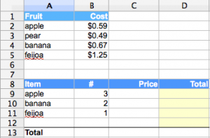
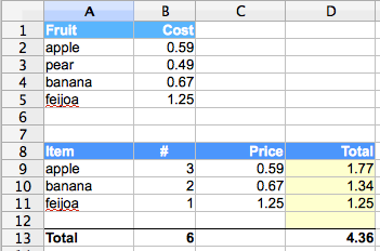
Here you can see both the initial list and the items and amount of each item I want to purchase.  Notice there’s no price showing up in my purchase list yet.  This is where the fun begins!  What I want to do is cross reference the item with the price from the list above.  For example, in cell C9, I want the function to answer the question “What is the cost of an apple?”.  Another way to put it is: “Please look at the item in A9.  Find that same item in the list from A2 to A5.  Once you’ve found that item, tell me what the value is from the B column.”

Fortunately, there’s a really easy way to get this information using the VLOOKUP function.

Simply put, the VLOOKUP function will allow you to search an array of cells to match a certain string and then return the result from the specified column.

In other word: VLOOKUP(<string to search for>; <array of cells to search>;<column from the array to return from>;<mode>).

In this example I would do:

=VLOOKUP(A9;A2:B5;2;0)

So let’s explain each section.  The first item.. the “string to search for” is A9.  This is the cell we’re going to look at.  In the case of row C9 we’re asking the vlookup function to search for the word “apple”.

So where do we want it to search?  Well, we have a price list, so we want it to search in that list, right?  We know apple is SOMEWHERE between A2 and A5.  So we should put that as the array, right?  Well, we could.. but the VLOOKUP function wouldn’t be able to return the information we want.  The way this function works is you pass it all the columns the function will be dealing with, then you specify which column it’s going to return from.  We’re looking for both the name and the price of it, so we enter BOTH columns in our search array: A2:B5

Then we enter the column we’re going to return the value from.  In this case, B2 is the value we want.. that’s in the second column, so we enter 2.

Finally, we tell the function that we don’t care about sort order, so we set the mode to 0.

So here’s the function that we enter in that cell:

=VLOOKUP(A9;A2:B5;2;0)

And what result do we get?

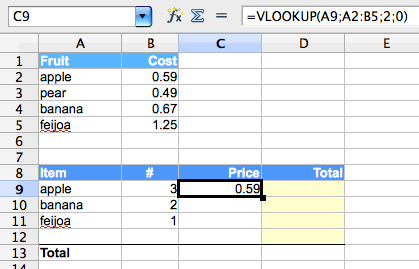
Pretty nifty, right?

Now, let’s copy that function and paste it into C10 and see what the result is.  Select C9, hit ctrl+c (or command+c on the mac).  Then go to C10 and hit ctrl+v (command+v on mac).  You should get the price of the banana.

This seems pretty straightforward, right?  just copy and paste.. copy and paste.  However, if you check out the function for cell C10, you’ll notice it’s changed.. the new function is:

=VLOOKUP(A10;A3:B6;2;0)

Did you see the difference?

The range that the function is searching has shifted down a cell.  Previously the range was A2:B5 and now it’s A3:B6.  This is because we didn’t explicitly say what the range should be.  When you enter a cell coordinate into a function, you have to tell open office calc whether or not to shift those cells when you copy and paste.  So how do we do that?

OOcalc has a nifty way of locking those cells down.. simply by entering a $ in front of either the Cell or the Row.  So in our case, we need to actually change our initial function in C9 to this:

=VLOOKUP(A9;A$2:B$6;2;0)

Now, if we copy that and paste it into C10 the function will look like:

=VLOOKUP(A10;A$2:B$6;2;0)

Notice that the search area stayed the same, ensuring we’re searching the correct cells, but the cell representing the string we’re looking for shifted appropriately (A9 to A10).

The next step is to simply copy that function to all the other slots in the C row that are appropriate.  In the case of our list, just to C11, but if you wanted to buy more produce.. add more lines and go for it!

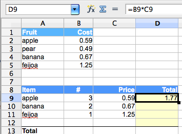
Now that we have the cost of each individual item, we need to tally up the cost based on the number of items we’re going to purchase.  To do this, select D9 and enter the following function:

=B9*C9

This will give us the actual cost of each item of fruit.  Copy that function to D10 and D11 and we’ll get the cost for each item we’re purchasing.

Finally, we want to sum up the total cost.  Here, we’ll use a simple SUM function to get the number of items we’re purchasing, and the total cost (minus taxes, shipping fees, etc.).

In B13 enter the following function:

=SUM(B9:B12)

And then copy that function to D13 and we’re done!

Now you can see how easy it is to build a list of items based on an initial price list.

In the next post, I’ll talk about how to extend this to creating a really useful way of tracking your Magic Card Collection and value.