Track your Magic The Gathering Collection with OOCalc – Part III

Now on to part III of my series on using OOCalc to track your Magic The Gathering card collection.  If you’ve missed parts 1 and 2, you may want to check them out, since part 3 builds upon those two bits.

Seriously, go read them.  You’ll be missing out on some pretty neato spreadsheet magic.

Go on, it’s okay.  I’ll wait.

…

Okay, you done?  Great!

In part III, we’re going to create the Collection bit of the spreadsheet where we get the value of our cards and calculate how much our collection is worth!

Oh man, can’t wait to sell the whole thing and buy a new Apple Tablet.

Yeah, I know they don’t “officially” exist yet, but I’m allowed to dream, aren’t I?

Okay, our current spreadsheet has two Sheets.. a blank Collection sheet, and our Pricelist that we downloaded and imported in part 2.

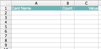
The Collection sheet is going to have the following columns: Card Name, Count, and Value. These should be pretty self explanatory, but just to make sure everyone is on the same page here..

Card Name will be the name of the card I want the value of.  It should match one of the names from the Pricelist sheet.

Count is the number of these cards that I have.

Value is going to be the associated price of the Card Name from the Pricelist sheet, multiplied by the Count.

So far so good?  Great!  Here’s an image of my spreadsheet so far with those headings placed at A1, B1, and C1.

Let’s go ahead and just enter the name of a card in A2.  For the fun of it, let’s pick a card that’s worth quite a bit of money.  How about.. Ancestral Recall from the Alpha series of cards.

Select A2 and type:

Ancestral Recall (A)

Obviously nothing happens yet, because we haven’t told C2 to get the price.  We’ll use the VLOOKUP function here to make the query.

Select C2 and type:

=VLOOKUP(A2;Pricelist.A2:B14317;2;1)

Remember.. the first field is the cell we want to grab and the second field is the array we’re going to search.  The third is the column within that array that we’re going to return, and the fourth is whether or not we’re sorting.  Since our pricelist is sorted alphabetially, we’re going to enter “1” for the sort value.

Notice something special in the second field.. we’re specifying a specific sheet to search for the array: Pricelist.A2:B14317.  This tells oocalc to go to a different sheet than the one we’re currently on.  If we didn’t do this, we would be searching the current sheet, and that wouldn’t do us any good at all.

We’re not quite finished yet, we still need to enter a Count.  Let’s pretend that we actually were really lucky and found 4 of these Ancestral Recall (A) cards.  Go ahead and enter 4 in B2.

Notice the value didn’t update, so we need to update the VLOOKUP function to multiply the value by the count.  Change VLOOKUP to:

=VLOOKUP(A2;Pricelist.A2:B14317;2;1) * B2

Not bad!  However, we still need to make a few more adjustments.  First, remember in part 1 when we copied and pasted our function it would offset the search values?  That’ll happen again if we copy C2 to C3.  Give it a shot and see what you get:

C2: =VLOOKUP(A2;Pricelist.A2:B14317;2;1) * B2

C3: =VLOOKUP(A3;Pricelist.A3:B14318;2;1) * B3

Some of the offsetting is fine.. A2 to A3 and B2 to B3 for example.  But the Pricelist.A2:B14317 being changed to Pricelist.A3:B14318 isn’t going to work.  Again, we need to use the $ symbol to lock down the cells we don’t want to adjust.

Change C2 to:

=VLOOKUP(A2;Pricelist.A$2:B$14317;2;1) * B2

Now you can copy and paste the field without it doing the wrong thing.

BUT you notice that if you DO paste into C3 without putting the name of anything in A3, you get a big lovely #N/A.  That means that the function is working, but it’s not returning a valid value.  That’s pretty ugly, isn’t it.  Let’s fix the display by telling the function to just return a blank string if there’s noting in A3.  We can do that using a Conditional!

We’re going to use an IF statement to check and see if A3 is blank.  If it is, we’ll display a blank value.  If not, then we’ll use our VLOOKUP function.

IF works like this:

IF ( Test; Then_value; Otherwise_value).

For example, if you had a value of “foo” in A1 and put this function in B1:

=if (A1=”foo”;”doo”;”darn”)

B1 would see that A1 does indeed = “foo”, so it would return “doo”.  If we did:

=if(A1=”poo”;”doo”;”darn”)

and A1 was still “foo”, then the expression would see that A1 didn’t equal “poo”, so it would return “darn”.

Does that make sense?

Here’s how we’re going to change our expression in C2:

=IF(A2=””;””;VLOOKUP(A2;Pricelist.A$2:B$14317;2;1) * B2)

Then copy and paste this into C3.  Notice the #N/A is gone?  That’s because we’re using the IF statement to check and see if A2 is blank.  Since it is, then this reuturns a blank string.  That looks much better!

Now let’s go ahead and enter another expensive card name in A3.. this time let’s use.. Badlands (A).

Notice the Value didn’t update.  That’s because we didn’t enter a count number.  If we simply change the value of count to 1, you’ll see the Value gets updated correctly:

Wouldn’t it be great if by default the count assumed it was always 1?  We can certainly do that by adding another function into our Value function.. MAX.

MAX will take a list of numbers and return the maximum number.  For example:

MAX(1;50) = 50

MAX(0;10;20;-5) = 20

MAX(.5;.7;150;10010) = 10010

Since we know that most of the time we’ll have 1 or more cards, we can assume that our anything lower than 1 should be returned as… 1.  So all we need to do is change the part of our function where we get the count from B2 to MAX(1;B2).  Then if B2 is 0, it will still return 1.  If it’s 10, then the funciton will return 10.  Sweet!

Go ahead and change C2 to the following function and then paste it into C3:

=IF(A2=””;””;VLOOKUP(A2;Pricelist.A$2:B$14317;2;1) * MAX(1;B2))

Notice that C3 now returns the proper value of the card.. and if you change B3, it will still add up correctly.

Nice!

The last bit of the tutorial is probably the coolest.. I can’t wait for you to see it! 🙂

You’ve probably noticed while scrolling through the list of card names that some of the Magic cards can be quite hard to spell..

It would be really easy to accidentally type in a name wrong and get the wrong value, or no value at all.  We could put in some crazy checking, but with 14,316 cards.. I’d much rather there was an easier way to search and enter card names.

Luckly, there is!

We can use the Validity feature of OOCalc!  It’s a great tool that lets you specify what exactly can be allowed to be entered into a cell.  We’ll use it on the Card Name column to ensure that only the cards shown in the Pricelist can be entered!

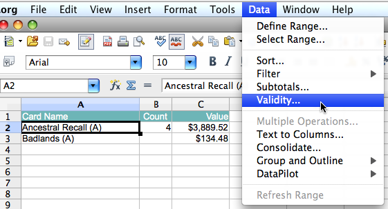
To do this, select A2.

Go Data -> Validity

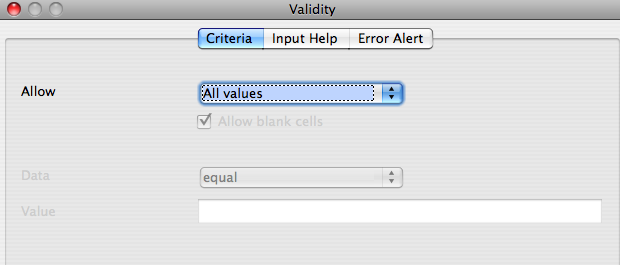
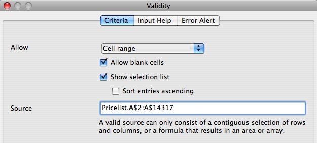
This will bring up the Validity window:

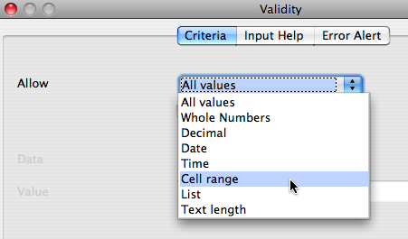
Here, you can tell oocalc exactly what type of item to allow in the cell.  The coolest thing is that you can choose a Cell Range.  That’s right.. we can pick the range of cells that are in our Pricelist that have the actual names of the cards.  Not only will this limit the input to only allow those names.. but it will actually create a dropdown option box so the person entering the names can just simply pick the one they want!

Yeah, that’s a LOT of italics, but it’s so cool!

Go ahead and tell it to allow a Cell Range:

Now enter the range:

Pricelist.A$2:A$14317

Make sure Show Selection List is on.

Click OK

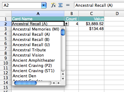
You’ll notice that there’s now a pulldown next to A2.  Go ahead and click on it.. you’ll get a pulldown of all the items in the pricelist!

Just pick the one you want and you’re done!

The rest is up to you.. just copy and the rows as you need them and you’ll be able to get the values of each card!

Enjoy!